Practical TurboQuant for Coders: Eliminating Bias with 1-Bit QJL and why you shouldn’t do it
It took me a looong time to write this second part. Was it the complexity of the math? Was it due to the summer holidays? Partially. It was actually due to wrong assumptions. It was my intuition that applying the QJL transform in addition to the TurboQuantMSE should lead to better search results. I was wrong. Read on to learn more.
If you read the first part of this series, we tackled the problem of “outlier” features in our BgGPT-3 embeddings. By applying a random rotation, we distributed the energy evenly across all dimensions, transforming the data into a beautiful, predictable normal distribution. This allowed us to precompute optimal Lloyd-Max quantization levels and compress our vectors down to 3 or 4 bits with near-zero memory overhead and minimal distortion.
However, the distortion we optimized was the mean squared error between the original and quantized vectors. In practice, what we care about is the dot product between the quantized embeddings and the query vectors (for example, in an LLM attention mechanism or a vector search index). It turns out that simply applying Lloyd-Max quantization to the rotated embeddings introduces a bias in the dot product approximations which can lead to sporadic errors and inconsistencies when used in real applications. Applying the Quantized Johnson-Lindenstrauss (QJL) transform to the residual error can eliminate this bias.
In order to evaluate the effectiveness of various quantization schemes, we can define the dot-product distortion as the difference between the true dot product and the approximated dot product:
\[(\mathbf{q} \cdot \mathbf{x}) - (\mathbf{q} \cdot \hat{\mathbf{x}})\]The bias would then be computed as the mean of this distortion over a large number of queries and embeddings. This is different from the mean absolute error.
\[\text{Bias} = \sum_{i=1}^{N} \frac{(\mathbf{q}_i \cdot \mathbf{x}_i) - (\mathbf{q}_i \cdot \hat{\mathbf{x}}_i)}{N}\] \[\text{MAE} = \sum_{i=1}^{N} \frac{|(\mathbf{q}_i \cdot \mathbf{x}_i) - (\mathbf{q}_i \cdot \hat{\mathbf{x}}_i)|}{N}\]The mean absolute error (MAE) is a measure of the average magnitude of the errors in a set of predictions, without considering their direction. The bias captures the systematic error in one direction. In other words, if our quantization consistently underestimates or overestimates the dot product, this will show up as a non-zero bias.
How do we fix this bias without bloating our memory footprint with scaling factors? Enter the second core innovation of the TurboQuant approach: the Quantized Johnson-Lindenstrauss (QJL) transform.
TurboQuant for dot-product approximations
The Johnson-Lindenstrauss (JL) Lemma states that we can project high-dimensional data into a lower-dimensional space while approximately preserving distances. The quantized version (QJL) takes this a step further - we only preserve the sign of the projection (i.e., +1 or -1), which can be stored in just 1 bit per dimension.
But why does this work? By applying QJL, we inject intentional, zero-mean mathematical randomness (stochasticity). Over millions of calculations (like computing LLM attention scores), these random errors average out to zero. It effectively wipes out the systematic bias using just 1 bit per dimension!
So, the dot product version of TurboQuant works like this:
- Apply the Lloyd-Max quantization using b - 1 bits to compress the main signal into a low-bit representation.
- Calculate the residual error left behind by the quantization process.
- Apply a random JL projection to the residual and quantize it down to 1 bit using the sign function.
- When approximating the dot product, we combine the base approximation from the main quantized vector with an error-correcting term derived from the 1-bit QJL residual.
Instead of using our entire bit budget to quantize the main embedding vector, we can use a small portion of it (just 1 bit per dimension) to encode the residual error left behind by the quantization process.
Does it work?
Only one way to find out - let’s try it.
Check the accompanying notebook for the full code. For brevity, I’ll just include selected highlights in this article.
Let’s start with the TurboQuantMSE class which implements the first part of the TurboQuant approach: random rotation + Lloyd-Max quantization. It’s quite simple: it just does a rotation and a quantization. The inverse operation is also straightforward: it dequantizes the indices back to the quantized values and applies the inverse rotation.
class TurboQuantMSE:

    def __init__(self, dim: int, bits: int = 4, rotation_matrix=None):
        self.dim = dim
        self.bits = bits
        self.R = rotation_matrix if rotation_matrix is not None else create_rotation_matrix(dim)
        self.thresholds, self.levels = compute_lloyd_max_thresholds(self.dim, self.bits, n_iter=100)

    def quantize(self, x: np.ndarray) -> np.ndarray:
        rotated = x @ self.R
        indices = np.digitize(rotated, self.thresholds).astype(np.uint8)
        return indices

    def dequantize(self, indices: np.ndarray) -> np.ndarray:
        reconstructed = self.levels[indices]
        return reconstructed @ self.R.T
Building on this, we can start work on the TurboquantIP class. We’ll do it bit by bit, so you can follow along and understand the inner workings of the algorithm. Let’s look at the constructor first:
class TurboQuantIP:

    def __init__(
        self,
        dim: int,
        bits: int = 3,
        rotation_matrix=None,
        jl_seed: int = 0,
    ):

        self.dim = int(dim)
        self.bits = int(bits)
        self.eps = 1e-12

        # Reuse TurboQuantMSE internally with b-1 bits
        self.base = TurboQuantMSE(dim=self.dim, bits=self.bits - 1, rotation_matrix=rotation_matrix)

        self.jl_matrix = sample_random_matrix(self.dim, seed=jl_seed).astype(np.float32)
        self.scale = np.sqrt(np.pi / 2.0) / self.dim
Most notably, we setup the base TurboQuantMSE quantizer with b-1 bits and create a random orthogonal matrix for the QJL projection. We also precompute the scale which will be needed for the inverse QJL operation.
Afterwards, we can consider the quantize method.
class TurboQuantIP:
    ...
    def quantize(self, x: np.ndarray):
        base_codes = self.base.quantize(x)
        base_hat = self.base.dequantize(base_codes)

        residual = x - base_hat
        residual_norm = np.linalg.norm(residual, axis=1)
        residual_dir = residual / np.maximum(residual_norm[:, None], self.eps)

        projected = residual_dir @ self.jl_matrix
        residual_sign = (projected >= 0).astype(np.uint8)

        return {
            "base_codes": base_codes,
            "residual_sign": residual_sign,
            "residual_norm": residual_norm,
        }
It’s more involved that the MSE version, but still quite simple: we quantize using the base quantizer, compute the residual, and then apply the QJL projection to the residual direction. The packed representation contains the base codes, the QJL signs, and the residual norm.
Now we can look at the dequantize method. It reconstructs the base approximation and adds the error-correcting term derived from the QJL projection of the residual:
class TurboQuantIP:
    ...
    def dequantize(self, packed) -> np.ndarray:
        x_hat = self.base.dequantize(packed['base_codes']).astype(np.float32)

        residual_norm = np.asarray(packed["residual_norm"], dtype=np.float32)
        qjl_residual = self._qjl_inverse(packed["residual_sign"])
        return x_hat + residual_norm[:, None] * qjl_residual

    def _qjl_inverse(self, residual_sign: np.ndarray) -> np.ndarray:
        sign = np.asarray(residual_sign, dtype=np.float32)
        z = 2.0 * sign - 1.0  # {0,1} -> {-1,+1}
        # In paper notation: Q_qj1^{-1}(z) = c * Pi^T * z
        return (self.scale * (z @ self.jl_matrix.T)).astype(np.float32)
The _qjl_inverse method maps the sign codes back to the original space using the precomputed scale and the transpose of the QJL matrix. The final reconstruction is a combination of the base approximation and the scaled QJL residual.
Now that we have the two classes implemented, we can evaluate their performance on a set of queries and embeddings. We will compare the dot product approximations and compute the bias and mean absolute error for both the TurboQuantMSE and TurboQuantIP methods.
We will compute the following metrics:
- Bias: The mean of the dot product distortion over all queries and embeddings.
- Std Dev: The standard deviation of the dot product error
- MAE: The mean absolute error of the dot product approximations.
- Hit Rate@k: is the true nearest neighbour of a query in the top-k results of the approximate search.
For a dataset, we will sample a subset of 100,000 embeddings from the BgGPT-3 model and a separate subset of 1000 query embeddings. Here are the results for different bit budgets:
| Metric | MSE (2 bits) | IP (2 bits) | MSE (3 bits) | IP (3 bits) | MSE (4 bits) | IP (4 bits) |
|---|---|---|---|---|---|---|
| Bias | -0.003484 | +0.000035 | -0.001024 | +0.000002 | -0.000293 | +0.000002 |
| MAE | 0.006397 | 0.007180 | 0.003111 | 0.004081 | 0.001575 | 0.002215 |
| Std Dev | 0.007773 | 0.008999 | 0.003836 | 0.005116 | 0.001978 | 0.002777 |
| Hit Rate@1 | 0.904 | 0.883 | 0.937 | 0.923 | 0.955 | 0.944 |
| Hit Rate@2 | 0.958 | 0.956 | 0.976 | 0.964 | 0.979 | 0.977 |
| Hit Rate@10 | 0.979 | 0.980 | 0.984 | 0.980 | 0.982 | 0.981 |
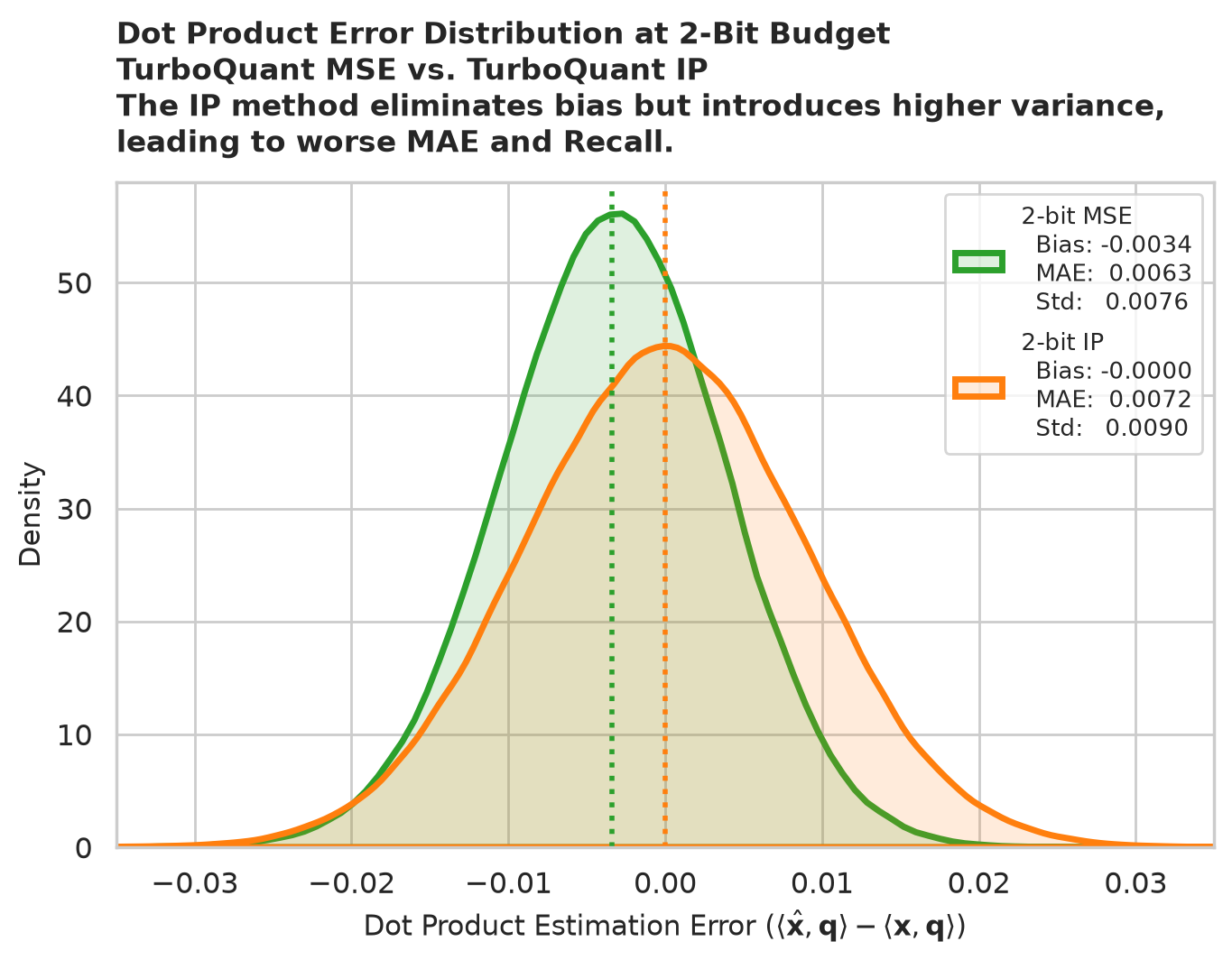
As can be seen from the table, the TurboQuantIP method effectively eliminates the bias in the dot product approximations, bringing it very close to zero. However, this comes at a cost in terms of higher mean absolute error and lower hit rates, especially for lower bit budgets.
I was surprised by this finding and kept coming back to my code - I was thinking there was a bug somewhere. My expectation was that the unbiased quantizer should lead to better search performance. It turns out that the TurboQuantIP method, while eliminating bias, actually results in slightly worse MAE and hit rates compared to the TurboQuantMSE method.
But why is that?
I dug deeper and found out that the answer lies in the nature of the QJL transform. By introducing stochastic noise to eliminate bias, we also introduce variance into the dot product approximations. This variance can lead to ranking swaps in the nearest neighbor search, which directly affects the hit rates. This is reflected by the higher stdev reported above.
It turns out I shouldn’t have been this surpised. This result is even present in the original TurboQuant paper, although it was not highlighted:
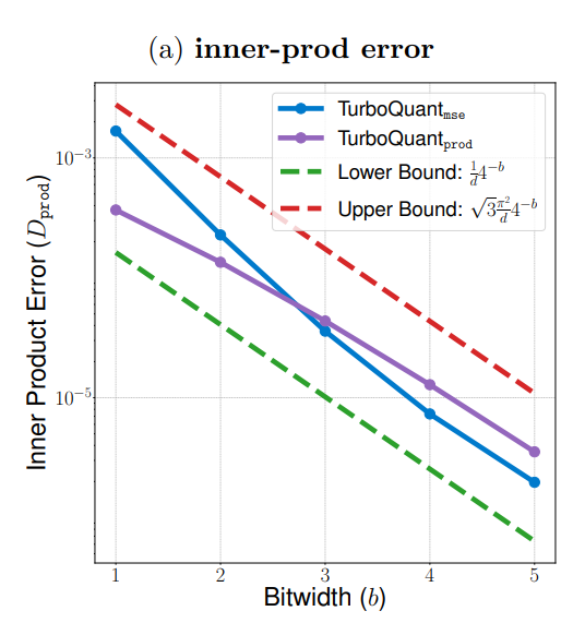
We can see that with bits $\ge$ 3, the reported inner product distortion is better for the MSE method than for the IP method.
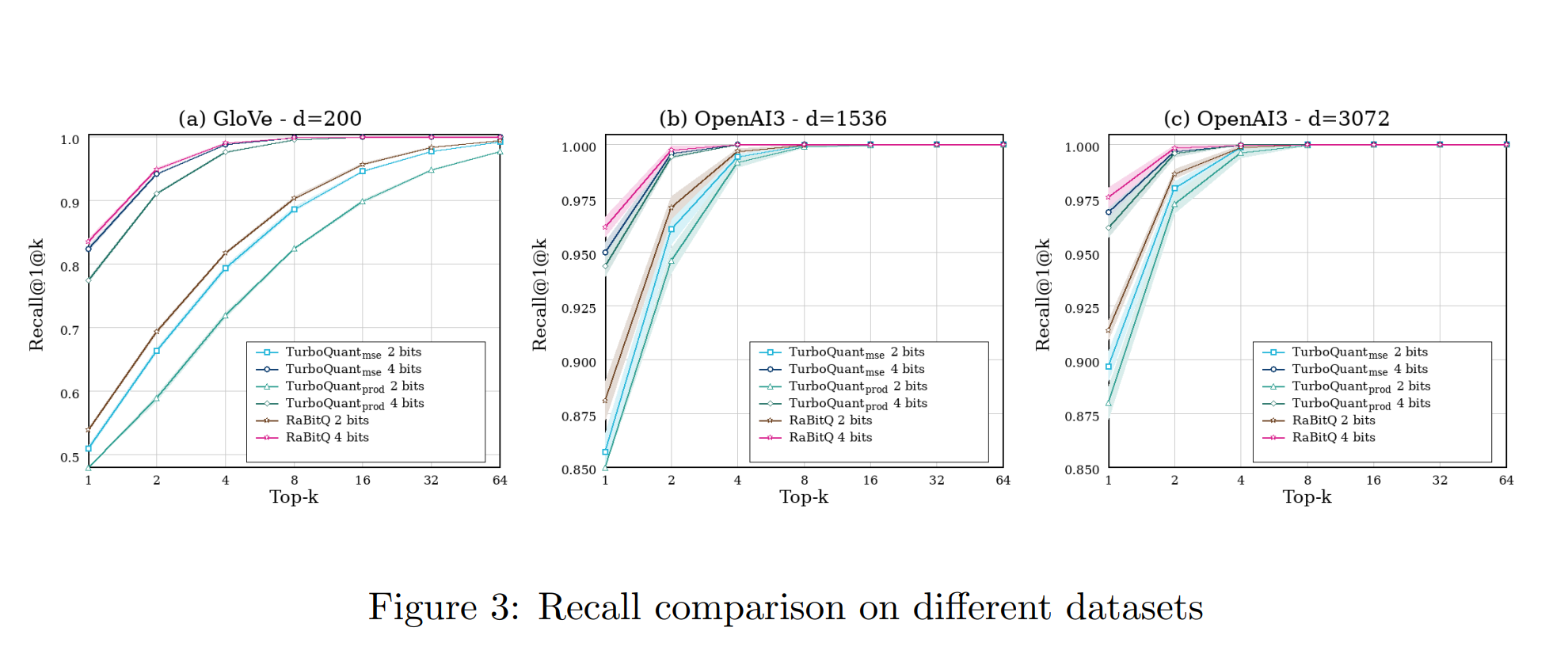
The same finding was also reported in Revisiting RabitQ and TurboQuant. We can see that across all three experiments, the TurboQuantMSE version achieves higher recall for the same bit budget.
So what does this mean? The Rank vs. Value Dilemma
This brings us to a fundamental engineering insight: your optimal quantization strategy depends entirely on whether your downstream task cares about ranking or absolute values.
1. Why Pure MSE Wins in Vector Search
In vector retrieval, we only care about retrieving the top-$k$ nearest neighbors.
- The TurboQuant MSE method achieves better MAE and lower variance in the dot product approximations, which translates to more stable rankings.
- In contrast, QJL introduces high-frequency, zero-mean stochastic noise. For candidates with close scores, this noise flips their order, causing ranking swaps and lowering Recall@k.
2. Why QJL Wins in Deep LLM Attention Layers
In LLM KV caches, inner products directly feed into non-linear activations:
- The bias of pure MSE acts like a persistent temperature multiplier inside the softmax function. This flattens attention weights, dilutes focus, and compounds layer over layer.
- Under sequence-length summation and multi-head averaging, unbiased QJL stochastic noise naturally cancels out to zero, preventing representation collapse in deep models.
Summary & Takeaways
To recap what we have built across this two-part series:
- Random Rotation + Lloyd-Max (TurboQuantMSE): Forces high-dimensional embeddings into a predictable Gaussian distribution, enabling optimal 2 to 4-bit compression with zero stored codebook overhead.
- 1-Bit QJL Residual Transform (TurboQuantIP): Uses a 1-bit sign projection to eliminate structural inner-product bias at the expense of higher variance.
You can find the full interactive experiments and benchmarking harness in the accompanying Jupyter Notebook on GitHub.
If you enjoyed this practical walkthrough, follow me on LinkedIn for more deep dives into the math and code behind modern AI!