If you’re like me, you were probably deeply impressed by the recent TurboQuant paper that claimed to be able to quantize large language models down to 4 bits without losing any accuracy. While most of the buzz has been around the applications in KV cache compression, I was more intrigued how this could be applied to vector/semantic search. The idea of being able to quantize the entire embedding space down to 4 bits without losing any precision could be a game-changer for building efficient vector databases and search engines.
So, what’s the problem? Those pesky embeddings that come out of deep learning models often have features with varying distributions. Some features might have extremely large values, while others are much smaller. This imbalance makes it challenging to quantize the embeddings effectively without losing important information.
So, how does TurboQuant solve this?
It applies a random rotation to the vectors. This way the energy of the outliers is spread evenly across all dimensions, making the distribution more suitable for quantization. Even more importantly, the distribution is known beforehand, so we can actually precompute the optimal quantization parameters. This means we don’t even need to calculate or store them!
In this article, we’re going to apply the first crucial part of the TurboQuant approach on the BgGPT-3 model as our guinea pig to illustrate these concepts in practice.
Extracting the Embeddings
For our experiments, we will use the word embeddings from the new BgGPT-3 model. These embeddings are the dense vector representations of words that the model uses to understand language.
Let’s first download the model:
from transformers import AutoProcessor, Gemma3ForConditionalGeneration
import torch

model_id = "INSAIT-Institute/BgGPT-Gemma-3-4B-IT"

processor = AutoProcessor.from_pretrained(model_id)
model = Gemma3ForConditionalGeneration.from_pretrained(
    model_id, device_map="auto"
).eval()
Then, we can extract the embeddings:
# extract the input embeddings
embeddings= model.model.get_input_embeddings().weight.detach().cpu().float().numpy()
embeddings.shape
> (262208, 2560)
Cool, so we’ve got a matrix of 262,208 tokens (the vocabulary size) and each token is represented by a 2560-dimensional vector.
For the math to work as expected, we need to L2 normalize the embeddings so that they are on the unit sphere. Warning: This is great if our ultimate goal is to use these embeddings for dot product approximation, but if we want to use them for euclidean distance-based search, we also need to preserve the norms. The authors also mention this in section 1.3 of the paper.
import numpy as np
E = embeddings/np.linalg.norm(embeddings, axis=1, keepdims=True)
For now, let’s just focus on the normalized embeddings in order to understand the benefits of TurboQuant.
Before & After Rotation: The Outlier Problem
In LLMs like BgGPT-3, activations often develop extreme “outlier” features. A specific latent dimension might have an unusually large mean or variance compared to the rest of the features. The TurboQuant paper states that applying a random rotation to the activations spreads the energy of these outliers across all dimensions, making the distribution more suitable for quantization. Furthermore, the paper claims that the distribution of the rotated activations is known beforehand, which allows for precomputing optimal quantization parameters.
First, we will apply the rotation and then we will see how it affects the distribution of the embeddings!
from scipy.stats import ortho_group

def random_rotation(matrix):
    R = ortho_group.rvs(matrix.shape[1])
    return matrix @ R

R = random_rotation(E)
Now we have the rotated embeddings in R. Let’s compare the distribution of the original embeddings E and the rotated embeddings R to see how the rotation has affected the outliers.
import seaborn as sns
import matplotlib.pyplot as plt
import seaborn as sns
sns.set_theme()
sns.set_style("white")


fig, ax = plt.subplots(2, 2, figsize=(14, 10), sharex=True)

# Define colors
original_color = "#5B5EA6"
rotated_color = "#4ECDC4"

# Original means
sns.stripplot(x=E.mean(axis=0), jitter=0.3, size=7, alpha=0.7, ax=ax[0,0],
              color=original_color, edgecolor="black", linewidth=0.5)
ax[0,0].set_title("Original Embeddings: Mean per Dimension", fontsize=12, fontweight='bold', pad=10)
ax[0,0].set_xlabel("Mean value", fontsize=11)
#ax[0,0].grid(True, alpha=0.3, axis='x')
ax[0,0].set_yticklabels([])

# Original stdev
sns.stripplot(x=E.std(axis=0), jitter=0.3, size=7, alpha=0.7, ax=ax[0,1],
              color=original_color, edgecolor="black", linewidth=0.5)
ax[0,1].set_title("Original Embeddings: Std Dev per Dimension", fontsize=12, fontweight='bold', pad=10)
ax[0,1].set_xlabel("Std Dev", fontsize=11)
#ax[0,1].grid(True, alpha=0.3, axis='x')
ax[0,1].set_yticklabels([])

# Rotated means
sns.stripplot(x=R.mean(axis=0), jitter=0.3, size=7, alpha=0.7, ax=ax[1,0],
              color=rotated_color, edgecolor="black", linewidth=0.5)
ax[1,0].set_title("After Rotation: Mean per Dimension", fontsize=12, fontweight='bold', pad=10)
ax[1,0].set_xlabel("Mean value", fontsize=11)
#ax[1,0].grid(True, alpha=0.3, axis='x')
ax[1,0].set_yticklabels([])

# Rotated stdev
sns.stripplot(x=R.std(axis=0), jitter=0.3, size=7, alpha=0.7, ax=ax[1,1],
              color=rotated_color, edgecolor="black", linewidth=0.5)
ax[1,1].set_title("After Rotation: Std Dev per Dimension (Equalized!)", fontsize=12, fontweight='bold', pad=10)
ax[1,1].set_xlabel("Std Dev", fontsize=11)
#ax[1,1].grid(True, alpha=0.3, axis='x')
ax[1,1].set_yticklabels([])

fig.suptitle("Effect of Random Rotation on Embedding Distribution", fontsize=14, fontweight='bold', y=0.995)
plt.tight_layout()
sns.despine(fig, left=True)
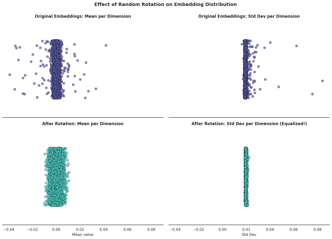
As can be seen from the picture: the rotation has effectively equalized the standard deviation across all dimensions and the outliers are virtually gone! Moreover, the stdev is as expected - $\frac{1}{\sqrt{d}} = \frac{1}{\sqrt{2560}} \approx 0.0197$. This means that the distribution of the rotated embeddings is now much more suitable for quantization, as there are no extreme outliers dominating the scale factor. Let’s plot the first 5 dimensions of the rotated embeddings to verify:
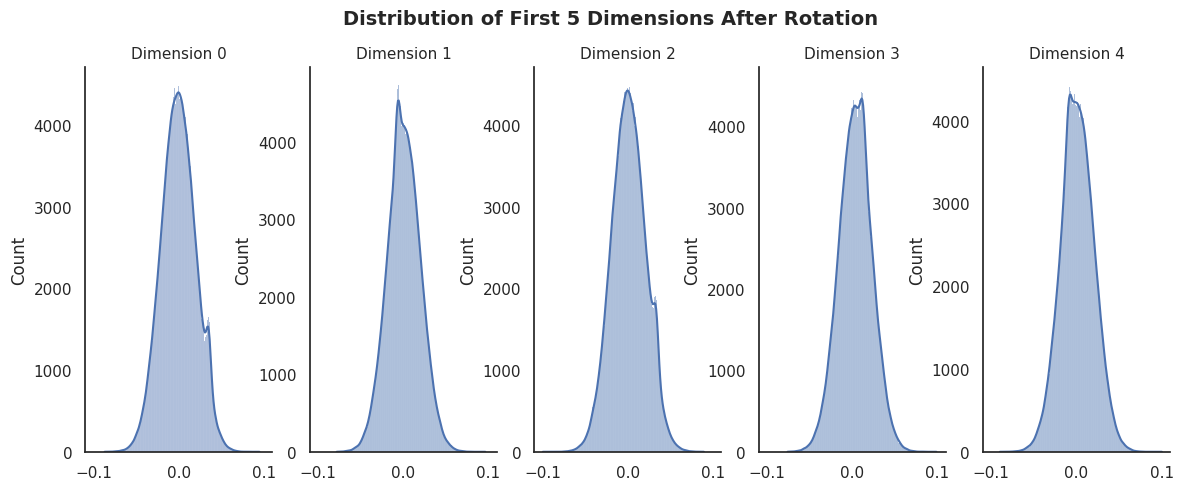
They all follow the familiar bell-shaped curve of a normal distribution, which is exactly what we wanted to achieve with the rotation!
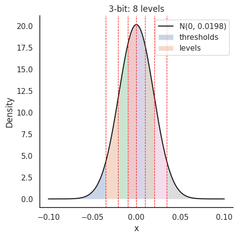
Now, since we know the distribution of each dimension of the rotated embeddings N(0, 1/d), we don’t need to train any quantizers - they can actually be precomputed as they depend only on d - the embedding dimension and b - the number of bits per dimension.
By applying the Lloyd-Max quantization algorithm for a Gaussian distribution, we can compute the optimal quantization levels and thresholds for our case:
| Bit Depth | Thresholds | Levels |
|---|---|---|
| 2-bit (4 levels) | -0.0194, -0.0000, 0.0194 | -0.0298, -0.0089, 0.0089, 0.0298 |
| 3-bit (8 levels) | -0.0345, -0.0207, -0.0098, -0.0000, 0.0098, 0.0207, 0.0345 | -0.0425, -0.0265, -0.0149, -0.0048, 0.0048, 0.0149, 0.0265, 0.0425 |
| 4-bit (16 levels) | -0.0474, -0.0364, -0.0284, -0.0217, -0.0158, -0.0103, -0.0051, 0.0000, 0.0051, 0.0103, 0.0158, 0.0217, 0.0284, 0.0364, 0.0474 | -0.0540, -0.0408, -0.0319, -0.0248, -0.0186, -0.0129, -0.0076, -0.0025, 0.0025, 0.0076, 0.0129, 0.0186, 0.0248, 0.0319, 0.0408, 0.0540 |
If we overlay the levels for b=3, we can see that we get more quantization levels around the mean, which is where most of the data points are, and fewer levels in the tails, which is exactly what we want for optimal quantization:
Summary
In this article, we explored the first crucial part of the TurboQuant approach - applying a random rotation to the embeddings to spread out the energy of the outliers and make the distribution more suitable for quantization. We saw how this rotation effectively equalizes the standard deviation across all dimensions and eliminates the extreme outliers, resulting in a much more quantization-friendly distribution. Moreover, since we know the distribution of the rotated embeddings, we can precompute the optimal quantization parameters using the Lloyd-Max algorithm for a Gaussian distribution.
But the puzzle doesn’t end here! In the next article, we will look at the second step of the TurboQuant approach - applying the Quantized Johnson-Lindenstrauss transform to further optimize the dot product approximations using a single bit!
If you enjoyed my practical walkthrough of the TurboQuant rotation step, follow me on LinkedIn, where I will share the next part and similar content.