Late Interaction Basics
I am fascinated with embeddings. Do you remember those word analogy examples? Paris is to France as Rome is to Italy? Fascinating. Embeddings have been present in one form or another in most of my work, blog posts and talks. Their ability to capture semantic relationships makes them a versatile tool that can be applied in many ways.
I also love full text search. I remember long nights in the university lab fiddling with tokenizers and inverted indices in an attempt to build a simple full text search engine. I think that’s what inspired me to pursue NLP.
We’re here today to talk about a technique which brings these two together: Late Interaction. Classical search systems may fail to understand the query or the documents in some major way - they have limited understanding of the context or the meaning of the document. On the other hand, vector search loses context in the aggregation/pooling step. Full attention reranking is too compute extensive to be used for search, so it is confined to the re-ranking step.
What if there was a middle ground? Late interaction search is an emergent technique which allows us to mitigate these problems.
This post will introduce the main ideas behind late interaction search and how it can improve on classical full text search and classical vector search.
Papers
The main papers we will focus on are:
- ColBERT: Efficient and Effective Passage Search via Contextualized Late Interaction over BERT
- ColBERTv2: Effective and Efficient Retrieval via Lightweight Late Interaction
Comparison
Please study the following graphic in detail. It shows the differences between full text search, vector search and late interaction search. For each search technique, we show how it functions during index time and during query time. If you click on the image, it will open in a new tab so you can explore it in full screen.
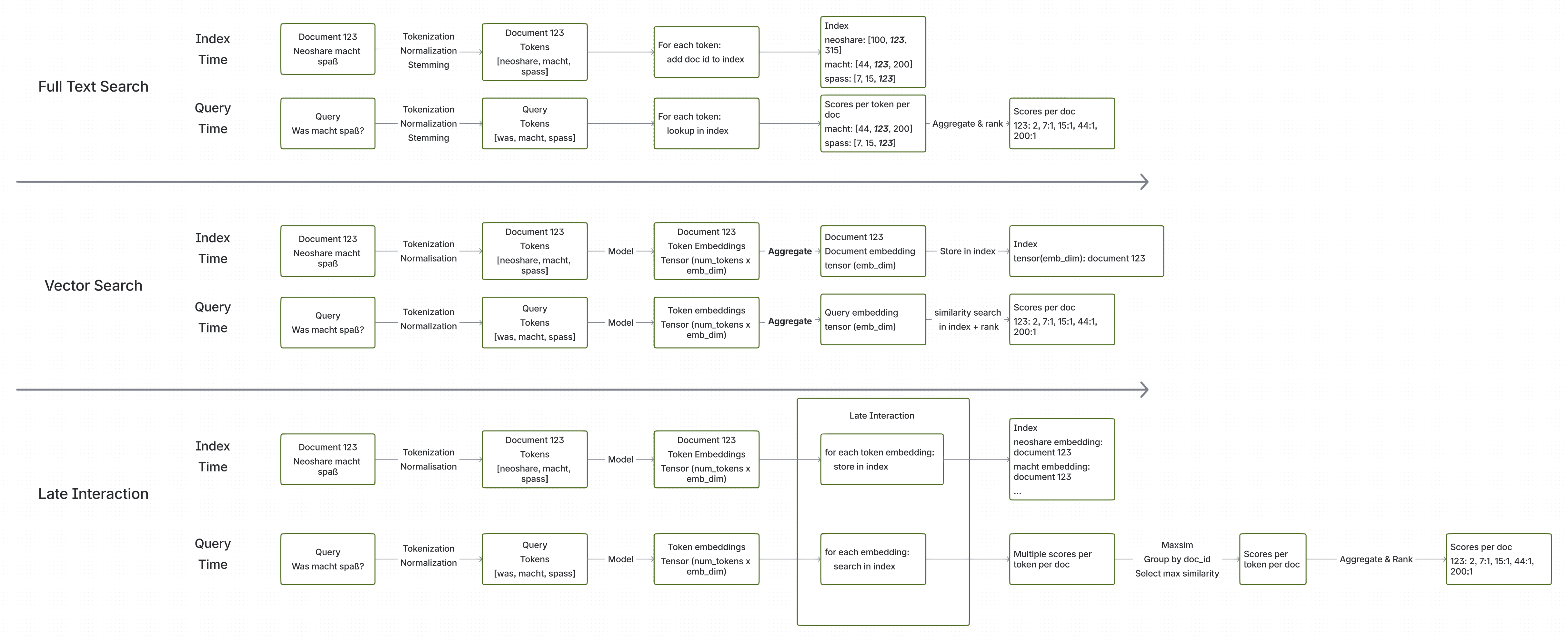
In the graphic we have three swimlanes, but they share a lot of common elements like tokenization, aggregation or ranking. Let’s walk through them one by one and highlight both the similarities and the differences. We will use a simple example document and query to illustrate the concepts.
Example Document:
{
    "document_id": "123",
    "text": "Neoshare macht Spaß"
}
Example Query:
{
    "query_text": "was macht spaß?"
}
Full Text Search
In full text search, we start with tokenization. It is common practice to also apply normalization, stopword removal and stemming/lemmatization at this point. Tokenization starts with a sentence and splits it into tokens. So “Neoshare macht Spaß” becomes [“neoshare”, “macht”, “spass”].
Afterwards, the algorithm updates the inverted index for each token. This means that we store an entry that the token “neoshare” appears in document 123, the token “macht” appears in document 123 and the token “spaß” appears in document 123. Of course, we do this for all documents in the corpus.
During query time, the query text goes through the same tokenization process. So “was macht spaß?” becomes [“was”, “macht”, “spass”]. Afterwards, we look up each token in the inverted index and retrieve the list of documents that contain each token. Finally, we aggregate the results and rank them based on some scoring function like TF-IDF or BM25.
This algorithm is simple, efficient, battle-tested and works well in many scenarios. However, it relies on the exact matching of tokens. If the query uses different words or synonyms, the search will probably fail to retrieve relevant documents.
The remaining two techniques aim to capture the semantic meaning of the text.
Vector Search
The key difference? Instead of exact token matching, we’re chasing semantic meaning.
In vector search, we employ an embedding model to convert the text into a dense vector representation. By embedding model, we usually mean a neural network that has been trained to produce vector representations of text that capture semantic meaning. Most of the latest embedding models are based on transformer architectures.
At index time, we start with the usual suspect: tokenization. For embedding models, it is less common to apply normalization, stopword removal and stemming/lemmatization here, as the embedding model can handle these aspects. Depending on the embedding model, tokenization may produce subword tokens or word pieces.
After tokenization, we pass the tokens through the embedding model to obtain their vector representations. Note that usually the embedding model produces a vector for each token. To obtain a single vector representation for the entire document, we apply an aggregation function like mean pooling or taking the vector corresponding to a special token like [CLS]. This results in a single vector for the entire document, which we then store in a vector database along with the document ID.
During query time, the query text goes through the same tokenization and embedding process to obtain its vector representation. We then perform a similarity search in the vector database to find the most similar document vectors to the query vector. The results are ranked based on their similarity scores.
By capturing semantic meaning, vector search can retrieve relevant documents even if they don’t contain the exact words used in the query. However, the aggregation step can lead to loss of important contextual information, as it compresses the entire document into a single vector. As documents get longer and more complex, this loss of context can become a significant problem.
This is where late interaction search comes into play! It combines the best of both worlds to mitigate the problems of both full text search and vector search.
Late Interaction Search
Here’s the big idea: What if we didn’t pool the token vectors into a single document vector? What if we indexed all the token vectors and used them for search?
In late interaction search, we use the same or similar embedding models to extract the semantic representations of the text. However, instead of aggregating the token vectors into a single document vector, we keep the individual token vectors. Let’s see how this works.
At index time, we start with - you guessed it - tokenization. Again, we usually don’t apply normalization, stopword removal and stemming/lemmatization here. After tokenization, we pass the tokens through the embedding model to obtain their vector representations. So far, it’s exactly like vector search.
However, this is where it gets interesting: instead of aggregating the token vectors into a single document vector, we store each token vector individually in the vector database along with the document ID. This means that for our example document “Neoshare macht Spaß”, we will store three separate vectors in the vector database, one for each token: “neoshare”, “macht”, and “spass”. Uh-oh, persisting a vector for each token can quickly take up a lot of space, but we will cover that later.
During query time, the query text goes through the same tokenization and embedding process to obtain its token vectors. So “was macht spaß?” becomes three vectors, one for each token: “was”, “macht”, and “spass”. At this point, we perform a similarity search for each query token vector in the vector database to find the most similar document token vectors. This is quite similar to the full text search approach, where we look up each token in the inverted index.
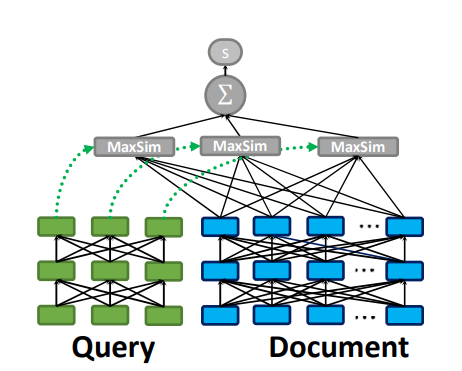
There is an important difference, though: in the inverted index we would get a single score per token per document, whereas here we could potentially get multiple similar token vectors per query token per document. To solve this issue, we simply take the maximum similarity score for each query token per document. This is called MaxSim.
Finally, we aggregate (sum) the maximum similarity scores for all query tokens to obtain a final score for each document. The documents are then ranked based on their final scores. This way each query token can contribute to the final score of a document based on its most similar token vector in that document.
The late interaction mechanism allows us to blend the strengths of both full text search and vector search. By keeping the individual token vectors, we retain more contextual information compared to vector search, which helps in understanding the nuances of the text. At the same time, by using vector representations, we can capture semantic meaning and retrieve relevant documents even if they don’t contain the exact words used in the query.
All of this comes at a cost, though. Storing individual token vectors can lead to significant storage overhead, especially for large corpora with long documents. Additionally, the vector lookup operations during query time are more computationally intensive compared to traditional full text search.
The next few sections will explore different aspects of late interaction search in more detail.
Late Interaction vs Attention
If we think about the computation involved in late interaction search, it stands somewhere between traditional vector search and full attention models like BERT.
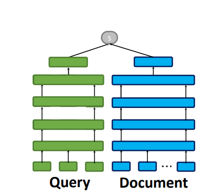
In vector search, we encode the query and the document separately. This allows us to precompute the embeddings for the documents and store them in a vector database. During query time, we only need to compute the embedding for the query and perform a similarity search in the vector database.
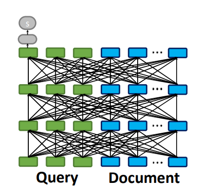
In full attention models like BERT, we concatenate the query and the document and pass them through the model together. This allows the model to attend to both the query and the document simultaneously, capturing complex interactions between them. However, this approach is computationally expensive, as we need to run the model for each query-document pair. This is why full attention models are usually only used for re-ranking a small set of candidate documents retrieved by a more efficient method first.
 Late interaction search strikes a balance between these two approaches. We still encode the query and the document separately, allowing us to precompute the document embeddings. However, when we perform the lookups for each query token vector, we are effectively approximating the attention scores between this query vector and all document token vectors.
This allows us to capture some of the interactions between the query and the document without breaking the budget. The next section will highlight how ColBert compares to full attention models in terms of effectiveness and efficiency.
Speed and quality
The authors of the ColBERT paper report the following results on the MS MARCO passage ranking task:
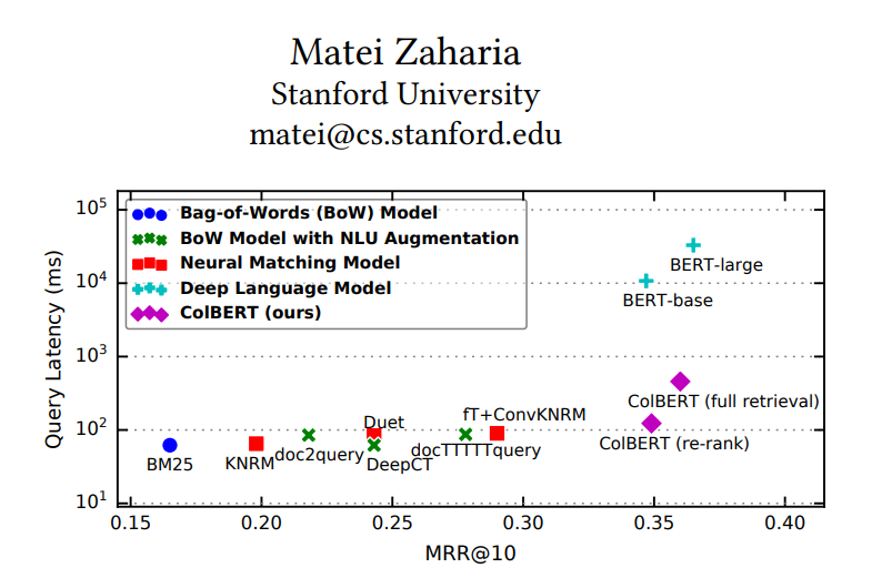
On the x-axis we have the quality, measured in MRR (Mean Reciprocal Rank). Higher MRR means better quality. On the y-axis we have the latency in milliseconds. Lower latency means faster search. Note that they y-axis is logarithmic, so small differences in the y-axis correspond to large differences in latency.
The classical BM25 method is in the bottom left corner. It is very fast, but has relatively low quality: we get responses in < 100ms, but the MRR is around 0.16. In contrast, the BERT-base and BERT-large models have much higher quality, with MMR around 0.35-0.36. However, they are also much slower - reported query latency is > 10,000ms. Can you imagine waiting 10 seconds for each search query? Not very practical.
So where does ColBERT come in? It combines the best of both worlds: it achieves MRR around 0.35, but it still responds in less than a second. The figure shows two variants: ColBERT(full retrieval) and ColBERT(re-rank). In the full retrieval mode, ColBERT is used as a standalone search engine, while in the re-rank mode, it is used to re-rank a set of candidate documents retrieved by a more efficient method first (e.g., BM25). The re-ranking mode is faster (~100ms) than the full retrieval mode(~600ms), but the quality is slightly lower as it depends on the initial candidate set. My gut feeling has a preference for the full retrieval mode, but you should experiment with both and see what works best for your use case.
Size
One of the main challenges with late interaction search is the storage overhead. Since we store individual token vectors for each document, the size of the index can grow significantly, especially for large corpora with long documents.
In the case of the MS Marco dataset:
- The original corpus has around 8.8 million passages.
- The raw text size is around 3GB.
- For classical vector search and a typical embedding model with embedding dimension 768, 8.8 million passages would require 27 GB of storage just for the token vectors.
- For late interaction, we need to do some math. According to the MS Marco paper, the average passage length is around 56 tokens with whitespace tokenization. This means that the total number of token vectors would be around 8.8 million * 56 = 492.8 million token vectors, which would require the staggering 63.1 GB of storage. With subwords, it will probably be two or three times higher! In fact, the ColBERT v2 paper reports that the Colbert index size for MS Marco is around 154 GiB.
It’s safe to say - this is a major limiting factor for the adoption of late interaction search in practice. So, how can we fix it? Here are a few ideas:
-
Pruning: the authors of ColBERT propose to prune the token vectors - drop tokens that are less informative like punctuation or stopwords. This is a drop in the ocean, but every bit helps. I think it can also help with the robustness of the system.
-
Quantization: instead of storing the full token vectors, we can apply quantization to reduce their size. This is the focus of the ColBERTv2 paper. They use an aggresive residual vector quantization technique to reduce the size of the token vectors by a factor of 6-10x. This allows them to shrink the entire index to around 25GiB, which is much more manageable and it’s equivalent to the size of a typical vector search index.
-
Clustering: as a compromise between storing a vector for each token and storing a single vector for the entire document, we can cluster the token vectors and only store the cluster centroids in the index. That way we can control the number of vectors per document and adjust it so it meets our quality, latency and storage requirements.
The chart below shows a comparison of the different storage requirements:

Thinking tokens / Query Augmentation
In the pre-reasoning models era, there was often a recommended technique to ask the model to explain its reasoning or solution. E.g. add “Let’s think step by step”. This allows the model to use more compute to come up with an answer - see the section “models need tokens to think” in Deep Dive into LLMs like ChatGPT by Andrej Karpathy.
In the ColBERT paper they suggest a similar approach: append a few
Let’s walk through an example:
- Query:
was macht spass - Tokenization:
[was, macht, spass, <pad>, <pad>, <pad>] - Embedding: tensor: 6 x emb_dim
- Vector store: 6 lookups (1 for each token)
- MaxSim aggregation
Note how we are adding three
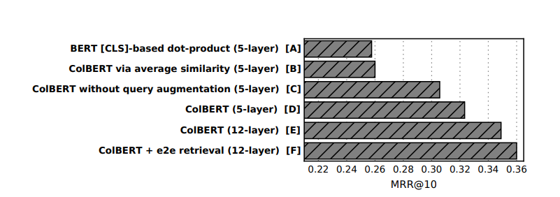
If we look at the ablation study from the ColBERT paper, we can see that adding the extra
Summary & Next Steps
Late interaction search is a powerful technique that combines the strengths of both full text search and vector search. By keeping the individual token vectors, we retain more contextual information compared to vector search, which helps in understanding the nuances of the text. At the same time, by using vector representations, we can capture semantic meaning and retrieve relevant documents even if they don’t contain the exact words used in the query.
All of this comes at a cost, though. Storing individual token vectors can lead to significant storage overhead, especially for large corpora with long documents. Additionally, the vector lookup operations during query time are more computationally intensive compared to traditional full text search. To mitigate these challenges, techniques such as pruning, quantization, and clustering can be employed to reduce the storage requirements and improve efficiency.
Where to go from here?
- Check out the ColBERT paper and the ColBERTv2 paper for more details
- Checkout ColPali: they use a similar framework, but embed image patches instead of text tokens - https://arxiv.org/abs/2407.01449
- Experiment with late interaction search in your own projects and see how it performs compared to traditional search
- Add me on LinkedIn if you liked this article!