Getting Started with Vector Search Indices: A Practical Introduction
In this blog post, we will explore several different types of FAISS (Facebook AI Similarity Search) indices - starting from Flat indices, to IVF indices, and finally to quantized indices. We will mostly focus on how they organize the data and how they perform search.
But before we dive into the details, let’s take a step back and understand what we’re trying to achieve. FAISS is a library for approximate nearest neighbor search - a problem that is more and more common with Retrieval Augmented Generation (RAG) and other applications. In those cases, documents are represented as vectors, and we want to find the most similar documents to a given query or anchor document.
Sometimes we have millions of documents, which makes it infeasible to compute the similarity between the query and all documents. This is where FAISS or other vector databases come in. They allow us to index the documents in a way that makes it possible to find the most similar documents quickly and efficiently. In the remainder of this post, we will explore some of the algorithms that allow us to do that.
Flat Index
The Flat index is the simplest and most straightforward way to store and search for vectors. The vectors are stored as-is in a flat array.
When a query comes in, the algorithm computes the distance between the query vector and every single vector in the dataset. As you can imagine, this can be quite slow for large datasets. There is also no memory savings or compression applied, so the index size is equal to the size of the dataset.
Let’s check out the code for a Flat index:
import faiss
import numpy as np
index = faiss.index_factory(128, 'Flat')
data = np.random.randn(64, 128)
index.add(data)
dist, indices = index.search(data[0][None], k=10)
dist, indices
> (array([[  0.     , 179.08739, 185.67009, 200.3658 , 206.49097, 206.8783 ,
         207.58463, 209.91669, 211.57022, 214.50839]], dtype=float32),
 array([[ 0, 11,  1, 53, 43, 12, 55, 23, 59, 10]]))
As soon as we add the data to the index, we can search for the nearest neighbors of a given vector - there is no training step. The search functionality simply computes the distance between the query vector and all vectors in the dataset and then returns the closest ones.
Inverted File Index (IVF)
IVF stands for Inverted File Index, and it’s a simple way to speed up searches by organizing data into clusters. Instead of comparing the query point to every single data point, an IVF index first narrows down the search to a smaller subset of the data.
This is done by clustering the data points into groups (or “cells”) and then only searching within the relevant clusters.
The code can look something like this:
import faiss
import numpy as np
index = faiss.index_factory(128, 'IVF8,Flat')

data = np.random.randn(512, 128)
# this time we need to train the index
index.train(data)
index.add(data)
dist, indices = index.search(data[0][None], k=10)
dist, indices
The IVF8 part means that the data is divided into 8 clusters. The Flat part means that within each cluster, the data is stored in a flat array (like in the Flat index).
If we have a larger dataset, we can increase the number of clusters to speed up the search even more.
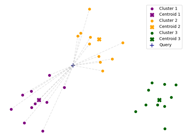
When we search for the nearest neighbors, the algorithm first finds the closest clusters to the query point and then searches only within those clusters.
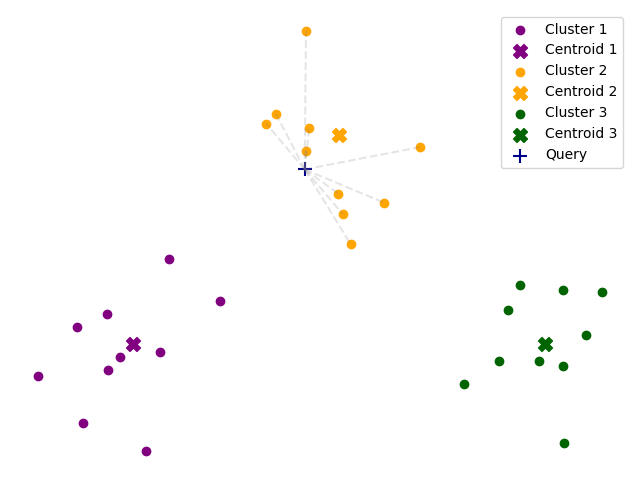
By default, FAISS looks up only the closest cluster, but this can lead to missing some of the closest neighbors. It
is possible to increase the number of clusters that are searched by setting the nprobe parameter.
index.nprobe = 4
dist, indices = index.search(data[0][None], k=10)
dist, indices
Scalar Quantization (SQ)
Scalar Quantization (SQ) is a compression technique that reduces the precision of vector components to save memory and speed up computations. Instead of storing each component as a 32-bit float, SQ maps the values to a smaller set of discrete levels using fewer bits (typically 8 bits or 4 bits). For example, with 8-bit quantization (SQ8), each component is mapped to one of 256 possible values, reducing memory usage by 75% compared to full precision. The trade-off is a slight loss in accuracy, but this is often acceptable given the significant performance gains.
How does a scalar quantizer work? First, it finds the minimum and maximum for each dimension and computes the “scale” as the difference between the maximum and the minimum. Then, items are mapped to an integer in the range [0, 255] according to the formula:
\[f(x) = \lfloor\frac{x - min}{max-min} * 255 \rfloor\]Example:
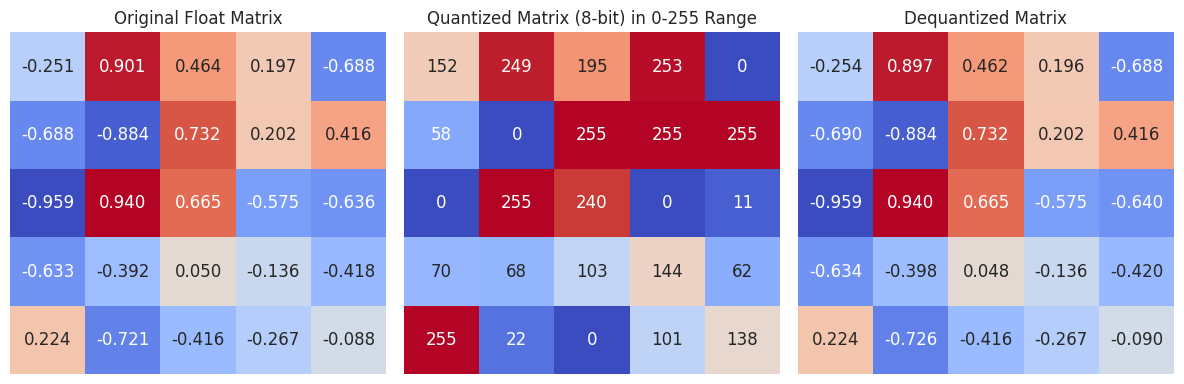
As you can see, the values are mapped to the range [0, 255] based on their relative position between the minimum and maximum values of each dimension. The minimum in each column corresponds to 0, the maximum corresponds to 255, and all other values are scaled accordingly.
It’s basically min-max normalization, but it maps to [0,255] instead of [0, 1]. With basic numpy, the implementation would be something like:
import numpy as np
#set seed
np.random.seed(42)

data = np.random.randn(512, 2)
min = data.min(axis=0)
scale = data.max(axis=0) - min

tfmd_data = np.floor((data - min) / scale * 255).astype(np.uint8)
tfmd_data[:5]
> array([[150,  92],
       [156, 160],
       [121,  88],
       [194, 129],
       [111, 120]], dtype=uint8)
To train a scalar quantizer in FAISS we can do the following:
import faiss
import numpy as np
index = faiss.index_factory(2, 'SQ8')
#set seed
np.random.seed(42)

data = np.random.randn(512, 2)
index.train(data)
Then, we can access the trained quantizer in index.sq.trained:
faiss.vector_float_to_array(index.sq.trained)
> array([-3.2412674, -2.4238794,  6.3201485,  6.276611 ], dtype=float32)
The first two numbers correspond to the minimums of their respective dimensions and the last two correspond to the scales.
We can also add the data to the index and inspect the codes:
index.add(data)
faiss.vector_float_to_array(index.codes).reshape(512, 2)[:5]
> array([[150,  92],
       [156, 160],
       [121,  88],
       [194, 129],
       [111, 120]], dtype=uint8)
In most cases, scalar quantization is used in combination with another indexing method, for example IVF8,SQ8. This allows us to combine the efficiency from the IVF clustering with the storage reduction from scalar quantization.
Interestingly, the SQ8 quantization is applied on the residuals of the vectors relative to their corresponding centroids.
Product Quantization (PQ)
Product Quantization (PQ) is a technique used to compress data points into smaller representations, making searches faster and more memory-efficient. In this method, the data points are divided into smaller sub-vectors, and each sub-vector is quantized separately.
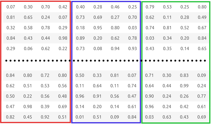
For example, suppose we have a collection of 128-dimensional vectors. We can split each vector into 4 sub-vectors of 32 dimensions each. Then, we can run k-means clustering independently on each of the sub-vector spaces to find a set of representative values (codebooks) for those parts of the vector. Afterwards, each vector can be represented as a combination of the indices of the codebooks for each sub-vector. So, our 128-dimensional vector can be represented as an array of 4 indices, with each index representing a centroid from the corresponding codebook.
How Does PQ Work?
At index time:
- Divide and conquer: Each data point $d$ (a high-dimensional vector) is split into m smaller sub-vectors $[d_0,d_1,..d_m]$
- Estimate codebooks: run k-means on each set of subvectors to find their centroids
- Store compact codes: Model each datapoint as the indices of the nearest centroid for each subvector
In the example below, we split the 12-dimensional vector into 3 subvectors of 4 dimensions each and run k-means on each subvector space.
At search time, product quantization works as follows:
- Split the query vector $\bold{q}$ into subvectors $[q_0,q_1,…, q_m]$
- Precompute distance tables: for each sub-vector $q_i$ and its corresponding codebook, compute the distance to all centroids. This creates M lookup tables containing .
- Lookup and sum distances: For each database vector calculate the distance to the query as the sum of the distances to its centroids
- Rank the vectors based on the approximated distances
At its extreme product quantization can even be used for 1-dimensional subvectors, similar to scalar quantization. Let’s see how this works so we can compare the two approaches:
import faiss
import numpy as np

d = 2 # dimension of the vectors
num_bits = 8 # number of bits per subvector
num_subvectors = 2 # number of subvectors

index = faiss.index_factory(d, f'PQ{num_subvectors}x{num_bits}')
#set seed
np.random.seed(42)

data = np.random.randn(512, d)
index.train(data)
codebooks = faiss.vector_float_to_array(index.pq.centroids).reshape(num_subvectors, 2**num_bits, d// num_subvectors)
codebooks.shape

> (2, 256, 1)
The returned centroids have shape (num_subvectors, $2^{num\_bits}$, d // num_subvectors).
Each codebook has shape [num_centroids, subvector_length ] where the number of centroids is $2^{num\_bits}$ and the subvector length is $\frac{d}{num\_subvectors}$.
In our case this corresponds to 2 codebooks each with 256 centroids of length 1.
Now we can add some data to index and decode it to inspect the changes
import pandas as pd
index.add(data[:2])
codes = faiss.vector_float_to_array(index.codes).reshape(2, -1)

def to_table(x):
    return pd.DataFrame(x).style.hide(axis=0).hide(axis=1)

display("Original Data", to_table(data[:2]))
display("Codes", to_table(codes))
display("Reconstruction", to_table(index.reconstruct_n(0, 2)))
display("Difference", to_table(data[:2] - index.reconstruct_n(0, 2)))

> 'Original Data'
0.496714	-0.138264
0.647689	1.523030
'Codes'
210	41
137	177
'Reconstruction'
0.495016	-0.138264
0.646183	1.526290
'Quantization error'
0.001698	-0.000000
0.001506	-0.003260
As you can see, the quantization introduces some error or loss in precision, but it has the potential for massive memory savings.
In practice, product quantization is used in combination with other indexing methods, such as IVF. Thus, the factory string
for creating a product quantization index would look like IVF8,PQ4x8, which means that the data is first clustered into 8 groups, and then each vector is quantized into 4 sub-vectors with 8 bits each.
In this case, the product quantization will be applied to the residuals of the vectors relative to their corresponding centroids in the IVF clusters. This helps decrease the variance. By combining these techniques, we can achieve
significant speedups and memory savings while still maintaining good search accuracy.
Summary
In this post, we explored several types of FAISS indices, including:
- Flat Index: The simplest index that stores vectors in a flat array and computes distances to all vectors during search.
- Inverted File Index (IVF): A more efficient index that clusters vectors into groups and searches only within relevant clusters, reducing the number of comparisons.
- Scalar Quantization (SQ): A compression technique that reduces the precision of vector components to save memory and speed up computations, often used in combination with IVF.
- Product Quantization (PQ): A technique that compresses data points into smaller representations by dividing them into sub-vectors and quantizing each sub-vector separately, allowing for efficient searches with reduced memory usage.
In terms of memory savings, we can provide the following comparison:
| Index Type | Memory per Vector | Storage for 1M Vectors (128d) | Memory Savings |
|---|---|---|---|
| Raw Vectors (32-bit float) | 512 bytes | 488 MB | 0% (baseline) |
| Flat Index | 512 bytes | 488 MB | 0% |
| IVF8,Flat | ~512 bytes* | ~488 MB* | ~0%* |
| SQ8 | 128 bytes | 122 MB | 75% |
| PQ4x8 | 4 bytes | 3.8 MB** | >99% |
*IVF adds a small overhead for centroids but doesn’t significantly reduce per-vector storage
**Plus overhead for codebooks (~4 KB for PQ4x8)
In a future post, we will explore more advanced indexing techniques, such as HNSW (Hierarchical Navigable Small World), OPQ (Optimized Product Quantization), and RVQ (Residual Vector Quantization).